How to Create a Slicer in an Excel Document

PlayLove

Editor

posted on 7 years ago — updated on 1 second ago

63
views

The slicer feature in Microsoft Excel allows you to be able to easily filter the data you want to see in a PivotTable. In versions of Excel before 2013, you had to use report filters to achieve a similar effect. However, it is not as easy to visualize report filters as it is to see what slicers are applied. Once created, slicers can be quickly applied in an intuitive way. Slicers can also be shared across multiple tables, removing the need for you to duplicate work.

Steps

Open Microsoft Excel. This can be done by using the desktop icon, through the Start menu, or by using the Quick Launch taskbar, depending on your computer preferences.

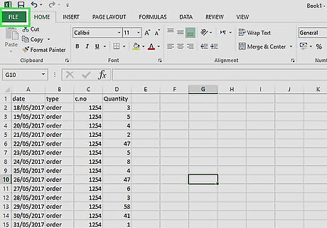
Load the Excel data file you want to visually filter in a pivot table. This can be done by clicking File in the upper left corner and then going to Open to select your data file.

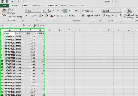
Highlight the data. You can highlight your data by either holding Ctrl+A or by left clicking with your mouse and dragging it over all the data.

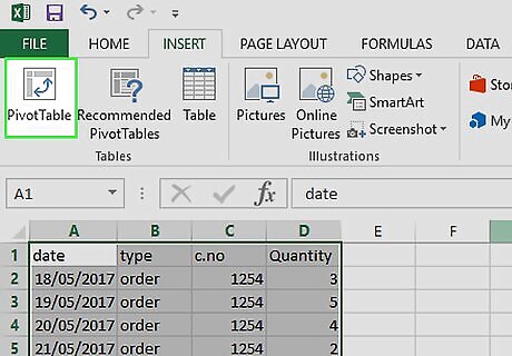
Select the PivotTable button.

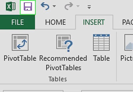
Save your progress. Left click on the disk icon in the upper left corner of your Excel file to save your progress.

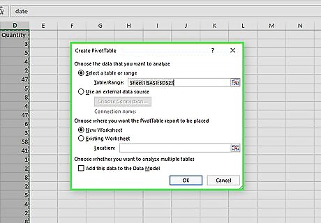
Choose your data range. In this menu, you can also choose the location of your pivot table. You can place it in an existing worksheet or create a new one.

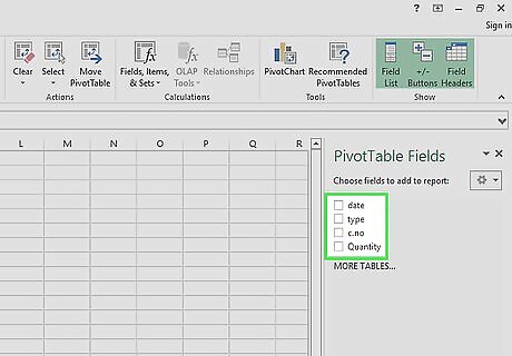
Check the boxes corresponding to the data sets you want included. You can check a single box or more than one.

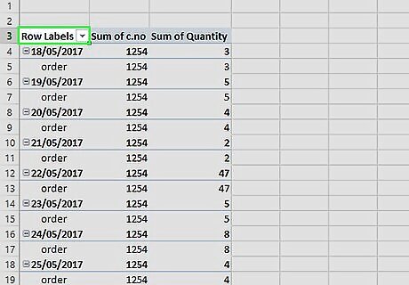
Pick your sorting options. Access the sorting options by clicking the table drop down menu

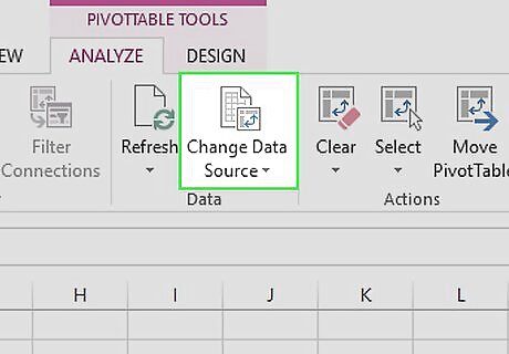
Change your data source. If you need to change the dimensions of your input range to accommodate more or less data you can find this from the “Options” ribbon under Change source data, you must select the table for this ribbon section to appear

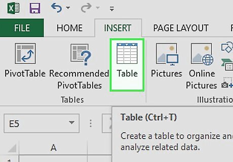
Insert a table within your data. You can then create a table to manage your data more easily. Highlight all your data, select insert, and then left click on the Table on the upper left side of your Excel sheet

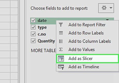
Right-click on pivot table field you want and choose “add as slicer”. On the right side of the Excel sheet, you can select the data field(s) you want to create a slicer for by checking the box next to the field. Then you right click on the field(s) you have chosen and click on Add as Slicer. By default, all slices of data will be selected.

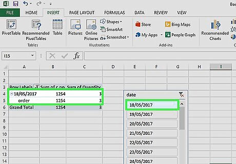
Select a single slice of data. To look at a single slice of data, simply left click the slice of data you want to look at.

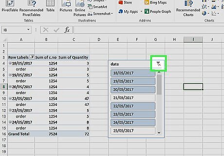
Select more than one slice of data. You can left click the multi-select button in Excel 2016 to select more than one slice of data. In Excel 2013, simply hold Ctrl and left click on all the slices of data you want to look at.