How to Combine Columns in Excel Without Losing Data

Using Flash Fill

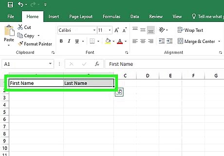
Know when to use Flash Fill. Flash Fill is the fastest way to combine the values of two columns (such as columns of separated first and last names). You'll teach Flash Fill how to merge the data by typing the first merged cell yourself (e.g., FirstName LastName). Flash Fill will sense the pattern and fill out the rest of the column. The two columns you're combining must be next to each other to use Flash Fill. Don't use Flash Fill if any of the following is true for your data (use the ampersand symbol or the CONCAT function instead): The columns you want to combine aren’t consecutive (e.g., combining columns A and F). You want to be able to make changes to the original columns and have those change automatically update in the merged column.

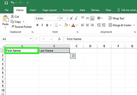
Add a blank column next to the columns you want to combine. In this example, let's say column A contains first names, column B contains last names, and that we want column C to contain first and last names combined. If column C isn't blank right now, right click the C column header and select Insert from the menu.

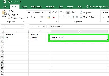
Type the full name into the first cell in column C. For example, if A1 contains Joe and B1 contains Williams, type Joe Williams into C1. Flash Fill can detect all sorts of patterns. For example, if column A contains area codes and column B contains phone numbers, you could type the area code and phone number into column C. You can even separate the contents of the columns with words or symbols, as long as you don't make the pattern too hard for Excel to understand. For example: A1 contains the area code 212 and B1 contains 555-1212, you could type (212) 555-1212 into column C and Excel should sense the pattern.

Press ↵ Enter or ⏎ Return. This teaches Flash Fill the pattern.

Start typing the next combined name into C2. As you type, you'll see that Excel suggest the next combination automatically. For example, if A2 is Maria and B2 is Martinez, Excel will suggest Maria Martinez.

Press ↵ Enter or ⏎ Return. This automatically combines the remaining cells from columns A and B into a single merged column C. You don't even have to drag down a formula—the two columns are now merged into one. If the column does not fill, press Control + E on the keyboard to activate Flash Fill manually. You can safely delete the original two columns if you'd like. The new column doesn't contain any formulas, so you won't lose the merged data.

Using the Ampersand Symbol

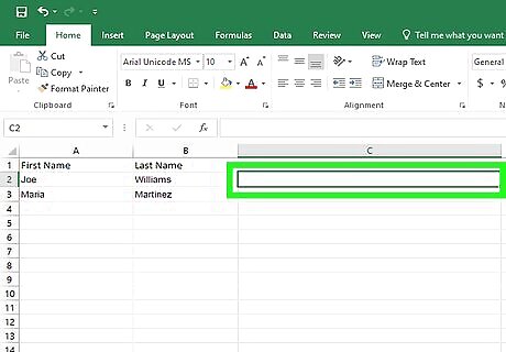
Click an empty cell near the columns you want to combine. This should be on the same row as the first row of data in the columns you're combining. Using the Ampersand & is another easy way to combine two columns. You'll create a simple formula using & symbols into the first cell, and then apply your formula to the rest of the data to merge the whole column.

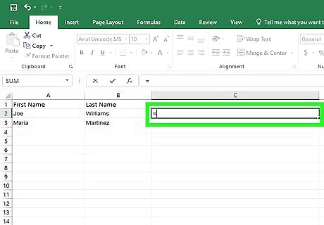
Type an equals sign = into the blank cell. This begins the formula.

Click the first cell in the first column you want to join. For example, if you're combining columns A and B, click A1. This adds the cell address to your formula.

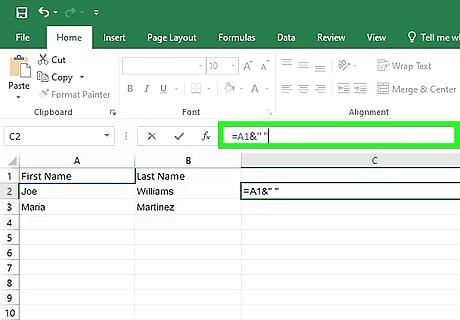
Type &" ". Place a single space between the two quotation marks. This tells the formula to add a space between the contents of the two columns. For example, if column A contains first names and column B contains last names, the " " ensures a space between the first and last names in the new column (e.g., "Joe Williams" instead of "JoeWilliams."

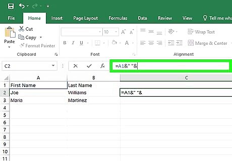
Type another &. This time, don't add any quotes or spaces.

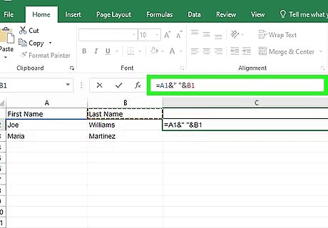
Click the first cell in the second column you want to merge. Now you'll have a formula that looks something like this: =A1&" "&B1 If you'd rather there not be a space between the words in the merged column, the formula would eliminate the " " and the second ampersand like this: =A1&B1 You could also place a symbol, word, or phrase inside of the quotes if you want to insert something between the two joined cells.

Press ↵ Enter or ⏎ Return. You've now merged the contents of the two cells at the top of each column.

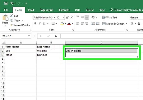
Click and drag the formula down the column. This merges the rest of the two columns. You can either click the cell and drag its bottom-right corner to the bottom of the columns, or double-click the square at the bottom-right corner of the cell to use autofill.

Convert the merged column into plain text. Because you used a formula to merge the two columns, the new column is just formulas, not text. If you want to delete the original columns and just keep the merged column, you'll need to do this to avoid losing data: Select all the combined data you've created. For example, C1:C30. Press Control + C (PC) or Command + C (Mac) to copy it. Right-click the first cell in the column you just copied. Select Paste Special and choose Values.

Using the CONCAT Function

Click an empty cell near the columns you want to combine. This should be on the same row as the first row of data in the columns you're combining. CONCAT works just like using the ampersand symbol. Its advantage is that it's easy to include in other formulas and is handy when making calculations. If you're just joining two columns by hand, using the ampersand is much easier.

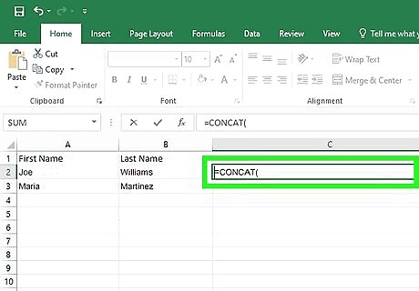
Type =CONCAT( into the blank cell. This begins the CONCAT formula. If you're using a version of Excel from before 2019, use CONCATENATE instead of CONCAT.

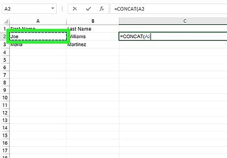
Click the first cell in the first column you want to join. For example, if you're combining columns A and B, click A1. This adds the cell address to your formula, which should now look something like this: =CONCAT(A1.

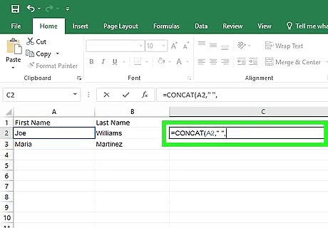
Type ," ",. Typing the first comma separates the first cell from " ", which adds a space between the two values. The second comma prepares you to select the second cell you're merging. You should now have a formula that looks something like this: =CONCAT(A1," ",

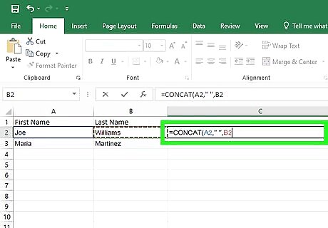
Click the first cell in the second column you want to merge and type a closed parenthesis ). Now you'll have a formula that looks something like this: =CONCAT(A1," ",B1). You could also place a symbol, word, or phrase inside of the quotes if you want to insert something between the two joined cells. Alternatively, if you want the merged text to appear without a space (e.g., JoeWilliams instead of Joe Williams), you could change the formula to =CONCAT(A1,B1).

Press ↵ Enter or ⏎ Return. This creates the formula and joins the two cells at the top of the columns.

Click and drag the formula down the column. This merges the rest of the two columns. You can either click the cell and drag its bottom-right corner to the bottom of the columns, or double-click the square at the bottom-right corner of the cell to use autofill.

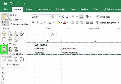
Convert the merged column into plain text. Because you used a formula to merge the two columns, the new column is just formulas, not text. If you want to delete the original columns and just keep the merged column, you'll need to do this to avoid losing data: Select all the combined data you've created. For example, C1:C30. Press Control + C (PC) or Command + C (Mac) to copy it. Right-click the first cell in the column you just copied. Select Paste Special and choose Values.