How to Calculate Difference in Pivot Table

Mdoggem

Editor

posted on 13 years ago — updated on 1 second ago

61
views

While pivot tables are very useful features for analyzing and explaining data in Excel, they can also be confusing to work with. Some functions, such as calculating differences, must be accomplished in a certain way if they are to work correctly. The process is not well explained within Excel's help feature, so here's how to calculate difference in pivot tables without using extraneous formulas.

Steps

Launch Microsoft Excel.

Open the spreadsheet containing the pivot table and source data you are working with.

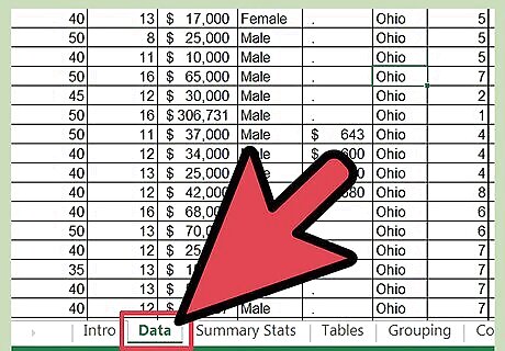
Select the worksheet tab containing the source data. This may, or may not, be the same sheet where your pivot table is located.

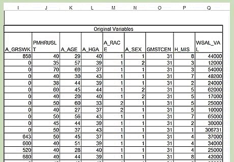
Determine the calculation you would like to add.

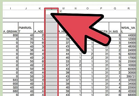
Insert a column for the calculated difference amounts. For instance, assume you want your pivot table to include a field showing the difference between column G and column H and both columns contain numerical fields. Right-click on column I and choose "Insert Column" from the pop-up menu. A column will be inserted to the right of column H and all columns of data beyond that column will be shifted one place to the right.

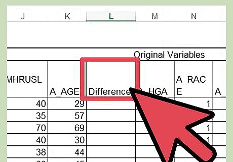
Enter a name for the column such as "Difference."

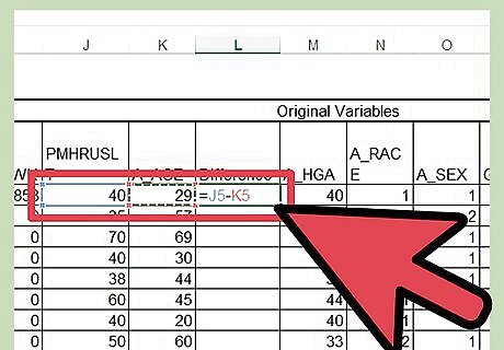
Create a formula in the first cell of your new column to calculate your differences. Using the above example, your formula would look like "=H1-G1" if you are subtracting column G from column H; "=G1-H1" if you are doing the reverse. Make sure you choose the correct syntax for your formula to return a positive or negative number as desired.

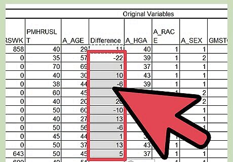
Copy and paste the formula through the rest of the new column.

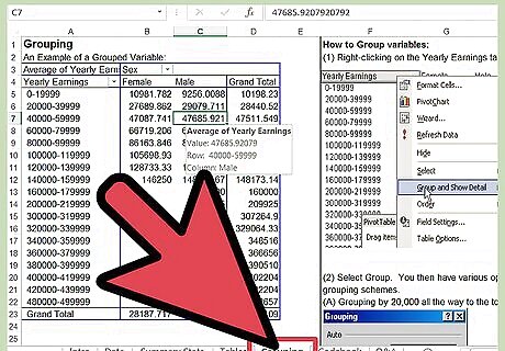
Click on the worksheet tab containing your pivot table, if it is different from the location of your source data.

Alter the source data for your pivot table. In Excel 2003, relaunch the pivot table wizard utility by clicking inside the pivot table and choosing "Wizard" from the pop-up menu. In Excel 2007 or 2010, click the "Change Source Data" button on the Pivot Tools Options tab. Either click and drag to highlight a new range or simply edit the range formula already in the "Range" field to include the following column.

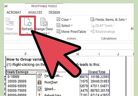
Refresh your pivot table by clicking the "Refresh" button.

Add the difference column to your pivot table by clicking the column name, dragging it and dropping it into the "Values" field of the pivot table wizard. You may need to reorder the column names in the "Values" section to make the columns appear in your pivot table in the correct order. You can click and drag from the "Values" section or directly within the pivot table to rearrange the order of your columns.